In the previous post (Latent Dirichlet Allocation), I’ve described the LDA process and how it can be applied on documents.
In this post I will explain how the probabilities can be estimated using collapsed Gibbs sampling.
Lets start with the LDA Probabilistic Graph Model.
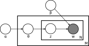
Where W is the sampled word from document, Z is the topic assigned by Document (d), θ is the Dirichlet distribution of d, α and β are the input of Dirichlets. More info about hyperparameters can be found this link.
So the only known variables are α, β, and w. All others (z, θ, and φ) are unknown. So based on the LDA graph we have:
p(w, z, θ, φ | α, β) = p(φ|β) p(θ|α) p(z|θ) p(w|φz)
The right side of the above conditional probability can be reached by the probabilistic graph model where each variable only depends on its parent nodes.
Inference
In LDA the we want to estimate latent variables (z, θ, and φ) based on known ones (α, β, and w). Thus we have:
p(w | α, β) can not be computed directly. So Gibbs Sampling is used to estimate latent parameters.
Collapsed Gibbs Sampling
Gibbs sampling is used to estimate p(x) = p(x1, …, xn) where there is no solution for p(x) but there are some forms of conditional probabilities. This method can be applied to LDA but there is a more simpler way to do this.
θ and φ can be calculated based on z where and
. In simple: θ is fraction words in document (d) where belong to the topic(z) and φ is the fraction of word (w) that belongs to topic (z) in the documents that w appeared in them.
So θ and φ can be out of computations. then we have to estimate:
Bayes conditional probability rules are coming: 🙂
Likehood and prior can be calculated easily. The computation process can be done by means of Expectation of Dirichlet distribution. For more information check these slides.